Nonstationary Kernels over Complex Terrain#
Download this notebook: nonstationary_terrain.ipynb
A stationary kernel uses one lengthscale and one variance everywhere. Over complex terrain this is a poor assumption. In Colorado, annual precipitation changes over a few kilometres in the Rocky Mountains, but only slowly over the Great Plains to the east. A stationary kernel must use one compromise lengthscale for both regions. Its intervals are then too narrow in the mountains and too wide on the plains.
Paciorek & Schervish (2006) used this example to motivate nonstationary kernels. In this notebook we
load the 1991–2020 annual precipitation normals at 247 Colorado stations,
let the variance and the lengthscale change with elevation, with the
VaryingAmplitudeandGibbskernels,compare these models with a stationary kernel on the marginal likelihood and on held-out stations, separately for the mountains and the plains, and
map the fitted lengthscale and amplitude.
from pathlib import Path

from jax import config
import jax.numpy as jnp
from jaxtyping import install_import_hook
import matplotlib.pyplot as plt
import numpy as np
import pandas as pd
import xarray as xr

config.update("jax_enable_x64", True)

with install_import_hook("gpjax", "beartype.beartype"):
    import gpjax as gpx
    from gpjax.kernels import location_functions
    from gpjax.parameters import val

gpx.plotting.use_style()
'ledger'
The data#
The NOAA U.S. Climate Normals give the mean annual precipitation for
1991–2020 at each station, with its location and elevation. The file in this
repository is a small netCDF subset for Colorado; see
docs/examples/data/_pull_reference_datasets.py for how it was made.
Precipitation is positive and skewed, so we model its logarithm, as Paciorek & Schervish did.
DATA = Path("data") if Path("data").exists() else Path("docs/examples/data")
stations = xr.open_dataset(DATA / "colorado_precipitation_normals.nc", engine="scipy")
stations
<xarray.Dataset> Size: 12kB
Dimensions:        (station: 247)
Coordinates:
  * station        (station) object 2kB 'USC00050102' ... 'USW00094082'
    name           (station) object 2kB ...
    lat            (station) float64 2kB ...
    lon            (station) float64 2kB ...
Data variables:
    precipitation  (station) float64 2kB ...
    elevation      (station) float64 2kB ...
Attributes:
    title:        Colorado annual precipitation normals, 1991-2020
    source:       NOAA NCEI U.S. Climate Normals 1991-2020 (annual/seasonal)
    references:   Palecki et al. (2021), U.S. Climate Normals 1991-2020, NOAA...
    license:      Public domain (work of the US Government).
Conventions: CF-1.8fig, (precip_ax, elev_ax) = plt.subplots(1, 2, figsize=(10, 3.6), sharey=True)
for ax, values, label, cmap in [
(precip_ax, stations.precipitation, "Annual precipitation (mm)", "viridis"),
(elev_ax, stations.elevation, "Elevation (m)", "cividis"),
]:
points = ax.scatter(stations.lon, stations.lat, c=values, s=14, cmap=cmap)
fig.colorbar(points, ax=ax, label=label)
ax.set_xlabel("Longitude")
ax.set_aspect(1 / np.cos(np.deg2rad(39.0)))
precip_ax.set_ylabel("Latitude")
Text(0, 0.5, 'Latitude')
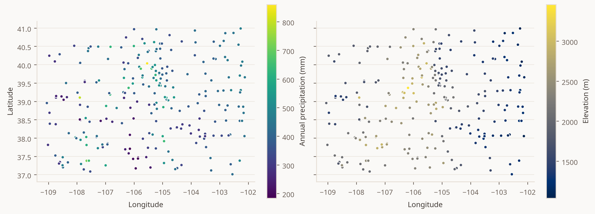
The wettest stations are high in the mountains in the west. The plains in the east are dry, and they change slowly. Elevation is the obvious covariate for the structure of the field.
We project the station locations to kilometres on a local plane, and we use units of 100 km so that the lengthscales start at a sensible value. We also standardise elevation, so that one unit of its weight is one standard deviation of elevation. The inputs have three columns: east, north and standardised elevation.
lat = stations.lat.to_numpy()
lon = stations.lon.to_numpy()
elevation = stations.elevation.to_numpy()

east = (lon - lon.mean()) * 111.32 * np.cos(np.deg2rad(lat.mean())) / 100.0
north = (lat - lat.mean()) * 110.57 / 100.0
elevation_scale = elevation.std()
standardised_elevation = (elevation - elevation.mean()) / elevation_scale

log_precipitation = np.log(stations.precipitation.to_numpy())
y_mean, y_scale = log_precipitation.mean(), log_precipitation.std()

X = np.column_stack([east, north, standardised_elevation])
y = ((log_precipitation - y_mean) / y_scale)[:, None]
data = gpx.Dataset(X=jnp.asarray(X), y=jnp.asarray(y))

mountains = elevation > 2000.0
print(f"{data.n} stations: {mountains.sum()} above 2000 m, {(~mountains).sum()} below")
247 stations: 112 above 2000 m, 135 below
Location functions#
A nonstationary kernel needs a parameter that has a value at each location.
GPJax calls this a location function. The module
gpjax.kernels.location_functions gives a
Constant and a log-linear Linear function, and you can subclass
AbstractLocationFunction for anything else.
A location function is not a mean function. A mean function describes the Gaussian process itself, but a location function describes its covariance. The two also have different contracts:
A location function evaluates one input point, and it selects its own columns with
active_dims. Here the base kernel measures distance over the east and north columns, while the location function reads only the elevation column.A location function returns a value on the log scale, and the kernel applies
exp. So the parameter is always positive, and a weight \(w\) multiplies the parameter by \(e^{w}\) for each unit of its column.
Linear starts with zero weights and no intercept. A model with these
functions therefore starts as exactly its stationary base kernel, and the base
kernel keeps the overall scale.
We compare four models. All of them use a Matérn-3/2 base kernel over east and north, a constant mean and Gaussian noise.
Stationary: the base kernel alone.
Varying amplitude: \(k(x, y) = \sigma(x)\,\sigma(y)\,k_0(x, y)\) with \(\log\sigma(x) = w_\sigma\,z(x)\), where \(z\) is standardised elevation.
Gibbs: the lengthscale is \(\ell_0\,\ell(x)\) with \(\log\ell(x) = w_\ell\,z(x)\). The marginal variance stays the same everywhere.
Both: a Gibbs kernel inside a varying-amplitude kernel.
def build_model(kind: str):
    base = gpx.kernels.Matern32(active_dims=[0, 1])

    def elevation_fn():
        return location_functions.Linear(active_dims=[2])

    if kind == "Stationary":
        kernel = base
    elif kind == "Varying amplitude":
        kernel = gpx.kernels.VaryingAmplitude(base, amplitude=elevation_fn())
    elif kind == "Gibbs":
        kernel = gpx.kernels.Gibbs(base, lengthscale=elevation_fn())
    elif kind == "Both":
        kernel = gpx.kernels.VaryingAmplitude(
            gpx.kernels.Gibbs(base, lengthscale=elevation_fn()),
            amplitude=elevation_fn(),
        )
    prior = gpx.gps.Prior(mean_function=gpx.mean_functions.Constant(), kernel=kernel)
    return prior * gpx.likelihoods.Gaussian(obs_stddev=0.3)


def negative_mll(model, data):
    return -gpx.objectives.conjugate_mll(model, data)


def fit(model, data):
    return gpx.fit_scipy(
        model=model, objective=negative_mll, train_data=data, verbose=False
    )


KINDS = ["Stationary", "Varying amplitude", "Gibbs", "Both"]
fitted = {}
log_marginal_likelihood = {}
for kind in KINDS:
    fitted[kind], history = fit(build_model(kind), data)
    log_marginal_likelihood[kind] = -float(history[-1])
What the fitted weights mean#
Because of the log link, each weight converts directly into a factor per 1000 m of elevation.
def weights_of(kernel):
    """The elevation weights of the amplitude and lengthscale functions."""
    weights = {}
    if isinstance(kernel, gpx.kernels.VaryingAmplitude):
        weights["amplitude"] = float(val(kernel.amplitude.weights)[0])
        kernel = kernel.base_kernel
    if isinstance(kernel, gpx.kernels.Gibbs):
        weights["lengthscale"] = float(val(kernel.lengthscale.weights)[0])
    return weights


per_km = 1000.0 / elevation_scale
for kind in KINDS[1:]:
    for name, weight in weights_of(fitted[kind].prior.kernel).items():
        print(
            f"{kind:18s} {name:12s} weight {weight:+.2f}: "
            f"x{np.exp(weight * per_km):.2f} per 1000 m"
        )
Varying amplitude  amplitude    weight +0.50: x2.55 per 1000 m
Gibbs              lengthscale  weight -0.99: x0.16 per 1000 m
Both               amplitude    weight -0.08: x0.86 per 1000 m
Both               lengthscale  weight -1.03: x0.15 per 1000 m
The Gibbs kernel learns a lengthscale that becomes much shorter at higher elevation, as we expected: precipitation changes over short distances in the mountains and over long distances on the plains. The amplitude alone learns a larger variance in the mountains. When both are present, most of the effect goes to the lengthscale.
Marginal likelihood and held-out stations#
The marginal likelihood is the first test. To test the predictions, we also use 5-fold cross-validation: we refit each model with one fifth of the stations held out, and predict those stations. We report the negative log predictive density (NLPD, lower is better) and the coverage of the 90% predictive intervals, separately for stations above and below 2000 m. A good model has coverage close to 0.90 in both regions.
folds = np.random.default_rng(0).permutation(data.n) % 5
z90 = 1.6449


def cross_validate(kind: str) -> dict:
    nlpd = np.zeros(data.n)
    covered = np.zeros(data.n, dtype=bool)
    error = np.zeros(data.n)
    for fold in range(5):
        train, test = folds != fold, folds == fold
        train_data = gpx.Dataset(X=data.X[train], y=data.y[train])
        model, _ = fit(build_model(kind), train_data)
        latent = model.predict(data.X[test], train_data, covariance="diagonal")
        mean = np.asarray(latent.mean)
        variance = (
            np.asarray(latent.variance) + float(val(model.likelihood.obs_stddev)) ** 2
        )
        residual = y[test, 0] - mean
        nlpd[test] = 0.5 * np.log(2 * np.pi * variance) + 0.5 * residual**2 / variance
        covered[test] = np.abs(residual) < z90 * np.sqrt(variance)
        error[test] = residual * y_scale
    return {
        "Log marginal likelihood": log_marginal_likelihood[kind],
        "NLPD": nlpd.mean(),
        "NLPD, mountains": nlpd[mountains].mean(),
        "NLPD, plains": nlpd[~mountains].mean(),
        "90% coverage, mountains": covered[mountains].mean(),
        "90% coverage, plains": covered[~mountains].mean(),
        "RMSE (log mm)": np.sqrt(np.mean(error**2)),
    }


scores = pd.DataFrame({kind: cross_validate(kind) for kind in KINDS}).T
scores.round(3)
| Log marginal likelihood | NLPD | NLPD, mountains | NLPD, plains | 90% coverage, mountains | 90% coverage, plains | RMSE (log mm) | |
|---|---|---|---|---|---|---|---|
| Stationary | -283.122 | 1.095 | 1.385 | 0.854 | 0.821 | 0.985 | 0.196 |
| Varying amplitude | -249.627 | 1.025 | 1.295 | 0.801 | 0.839 | 0.874 | 0.192 |
| Gibbs | -217.916 | 0.876 | 1.203 | 0.605 | 0.866 | 0.822 | 0.174 |
| Both | -217.757 | 0.879 | 1.195 | 0.618 | 0.875 | 0.815 | 0.173 |
The results agree with Paciorek & Schervish (2006):
The marginal likelihood improves strongly. The Gibbs kernel is much better than the stationary kernel, with only one more parameter.
The uncertainty becomes calibrated by region. The stationary kernel uses one compromise lengthscale. Its intervals are too narrow in the mountains and much too wide on the plains. The Gibbs kernel moves the mountain coverage towards 0.90. On the plains, the coverage changes from much too wide to slightly too narrow. The held-out NLPD falls in both regions, which shows that the predictive distributions are better overall.
The error falls less. The RMSE improves, but by less than the NLPD. Paciorek & Schervish also found that the main gain is in the likelihood and the uncertainty, not in the point predictions.
The varying amplitude alone helps less than the Gibbs kernel. Here the main nonstationarity is in the correlation length, not in the variance.
Maps of the fitted lengthscale and amplitude#
The lengthscale of the Gibbs kernel at each station is \(\ell_0 e^{w_\ell z(x)}\). We plot it in kilometres, together with the amplitude \(\sigma(x) = e^{w_\sigma z(x)}\) from the model with both functions.
both = fitted["Both"].prior.kernel
gibbs = both.base_kernel
lengthscale_km = (
    100.0
    * float(val(gibbs.base_kernel.lengthscale))
    * np.exp(np.asarray([gibbs.lengthscale(x) for x in data.X]))
)
amplitude = np.exp(np.asarray([both.amplitude(x) for x in data.X]))

fig, (ls_ax, amp_ax) = plt.subplots(1, 2, figsize=(10, 3.6), sharey=True)
for ax, values, label in [
    (ls_ax, lengthscale_km, "Lengthscale (km)"),
    (amp_ax, amplitude, "Amplitude multiplier"),
]:
    points = ax.scatter(stations.lon, stations.lat, c=values, s=14, cmap="magma")
    fig.colorbar(points, ax=ax, label=label)
    ax.set_xlabel("Longitude")
    ax.set_aspect(1 / np.cos(np.deg2rad(39.0)))
ls_ax.set_ylabel("Latitude")
Text(0, 0.5, 'Latitude')
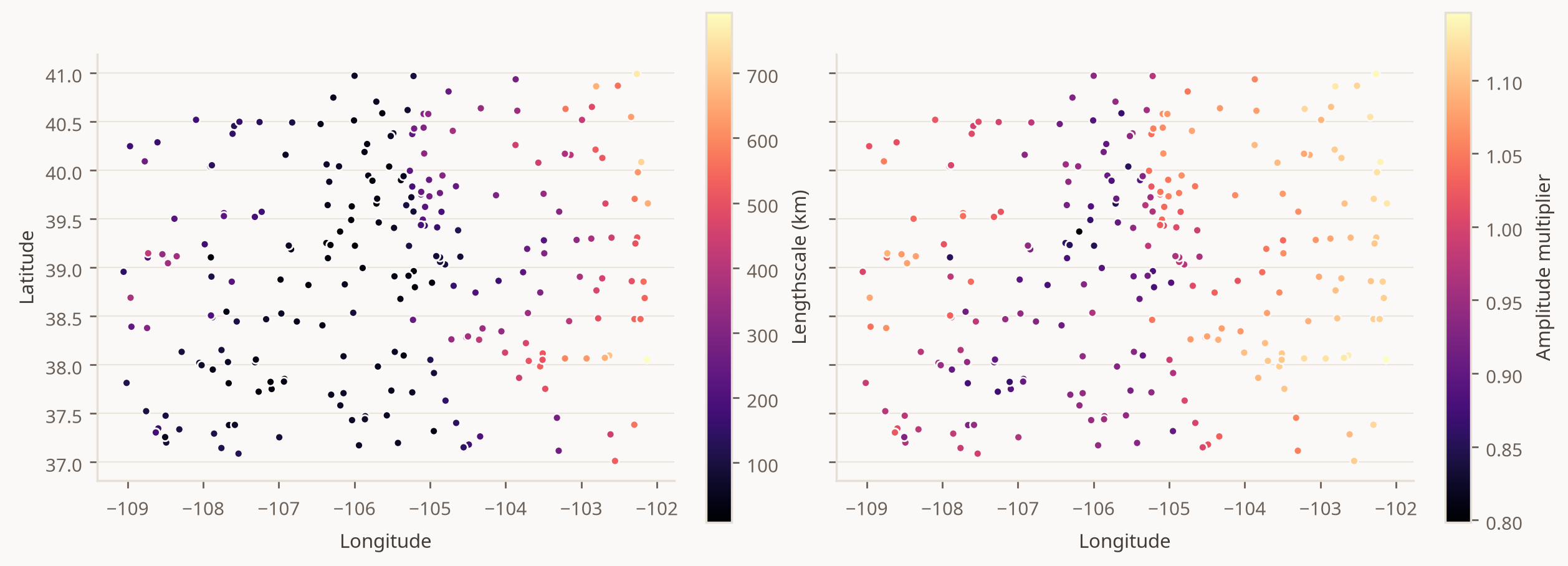
The lengthscale is a few tens of kilometres along the high ranges and a few hundred kilometres on the eastern plains.
Notes#
Valid base kernels. The Gibbs construction is positive definite only for an isotropic radial base kernel: RBF, the Matérn kernels, RationalQuadratic or PoweredExponential.
Gibbsraises aTypeErrorfor other kernels.VaryingAmplitudeaccepts any base kernel that evaluates one pair of points at a time.Extrapolation. Because of the log link, the lengthscale and the amplitude change exponentially with the covariate. Outside the range of elevations in the data, they can become very large or very small. Keep the predictions inside the range of the covariate.
Elevation as an input. You can also give elevation to the base kernel as a third distance column. This is a different idea: it makes stations at different elevations less correlated. It combines with the location functions, and on these data the combination is slightly better again.
Cost. The location function runs once for each row of a kernel matrix, so a nonstationary kernel costs about the same as its base kernel.
Pathwise sampling. These kernels have no spectral density, so
sample_approxdoes not support them. Sample from the predictive distribution instead.
References#
Gibbs, M. N. (1997). Bayesian Gaussian processes for regression and classification. PhD thesis, University of Cambridge.
Paciorek, C. J. and Schervish, M. J. (2006). Spatial modelling using a new class of nonstationary covariance functions. Environmetrics 17, 483–506.
Palecki, M. et al. (2021). U.S. Climate Normals 1991–2020. NOAA National Centers for Environmental Information.