Space–Time Modelling of Winter Temperature#
Download this notebook: spacetime_temperature.ipynb
A simple space–time kernel is separable: it is the product of a kernel in space and a kernel in time. Then the spatial correlation has the same shape at every time lag. Weather does not behave like this. A large anomaly, for example a blocking high over Scandinavia, persists for many days, while a small anomaly is gone after one or two days. So the spatial correlation between two days that are far apart comes mostly from the large anomalies, and it is broader than the spatial correlation on the same day.
The Gneiting kernel (Gneiting, 2002) models this
with one interaction parameter. In this notebook we fit it to daily
temperature anomalies over Europe in the winter of 2019, and compare it with
its separable version on the marginal likelihood and on held-out data.
import os
from pathlib import Path

from jax import config
import jax.numpy as jnp
from jaxtyping import install_import_hook
import matplotlib.pyplot as plt
import numpy as np
import pandas as pd
import paramax
import xarray as xr

config.update("jax_enable_x64", True)

with install_import_hook("gpjax", "beartype.beartype"):
    import gpjax as gpx
    from gpjax.parameters import val

gpx.plotting.use_style()

# Smoke-render flag: set GPJAX_DOCS_CI=1 to shrink the optimiser for fast CI builds.
ci = os.environ.get("GPJAX_DOCS_CI") == "1"
max_iters = 25 if ci else 500
The data#
We use daily near-surface air temperature from the NCEP-NCAR Reanalysis 1
(Kalnay et al., 1996), from 1 January to 1 March 2019. The anomaly is the
daily value minus the 1991–2020 mean for that day of the year. The file in
this repository is a coarse subset: 35 grid cells, 7.5° apart in latitude and
10° apart in longitude, over Europe and the north-east Atlantic. See
docs/examples/data/_pull_reference_datasets.py for how it was made.
DATA = Path("data") if Path("data").exists() else Path("docs/examples/data")
field = xr.open_dataset(DATA / "ncep_europe_winter_2019.nc", engine="scipy")[
    "tas_anomaly"
]
field
<xarray.DataArray 'tas_anomaly' (time: 60, lat: 5, lon: 7)> Size: 8kB
[2100 values with dtype=float32]
Coordinates:
  * time     (time) datetime64[ns] 480B 2019-01-01 2019-01-02 ... 2019-03-01
  * lat      (lat) float32 20B 70.0 62.5 55.0 47.5 40.0
  * lon      (lon) float32 28B -20.0 -10.0 0.0 10.0 20.0 30.0 40.0
Attributes:
    long_name:  Daily near-surface air temperature anomaly (sigma 0.995) agai...
units: Klimit = float(np.abs(field).max())
fig, axes = plt.subplots(1, 4, figsize=(12, 2.8), sharey=True)
for ax, index in zip(axes, [0, 7, 14, 21], strict=True):
image = field.isel(time=index).plot(
ax=ax, cmap="RdBu_r", vmin=-limit, vmax=limit, add_colorbar=False
)
ax.set_title(str(field.time.values[index])[:10])
ax.set_ylabel("Latitude" if index == 0 else "")
ax.set_xlabel("Longitude")
fig.colorbar(image, ax=axes, label="Anomaly (K)")
<matplotlib.colorbar.Colorbar at 0x7fb5e39454d0>
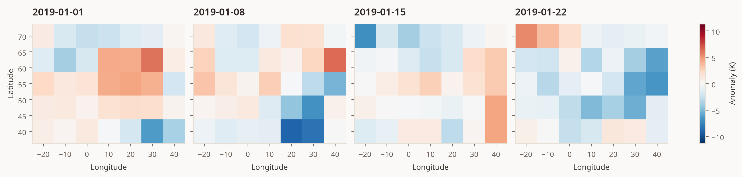
The anomalies are up to several thousand kilometres wide, and the pattern changes from one week to the next.
Inputs and a held-out gap#
The inputs have three columns: the day number, and east and north positions in units of 1000 km on a local plane. We hold out 20% of the grid cells for the middle third of the period. This is like a gap in the record of some stations, which a model must fill from their neighbours in space and in time.
lat, lon = np.meshgrid(field.lat, field.lon, indexing="ij")
east = np.deg2rad(lon - lon.mean()) * 6371 * np.cos(np.deg2rad(lat.mean())) / 1000
north = np.deg2rad(lat - lat.mean()) * 6371 / 1000

n_days, n_cells = field.sizes["time"], lat.size
day = np.repeat(np.arange(n_days), n_cells).astype(float)
cell = np.tile(np.arange(n_cells), n_days)
X = np.column_stack([day, east.ravel()[cell], north.ravel()[cell]])
y = field.to_numpy().astype(np.float64).reshape(-1)

held_cells = np.random.default_rng(0).choice(n_cells, n_cells // 5, replace=False)
in_gap = (day >= n_days // 3) & (day < 2 * n_days // 3)
test = np.isin(cell, held_cells) & in_gap
train = ~test

y_mean, y_scale = y[train].mean(), y[train].std()
y = (y - y_mean) / y_scale
train_data = gpx.Dataset(X=jnp.asarray(X[train]), y=jnp.asarray(y[train, None]))
print(f"{train.sum()} training points, {test.sum()} held-out points")
1960 training points, 140 held-out points
The Gneiting kernel#
For a spatial separation \(h\) and a time lag \(u\), the kernel is
where \(d = 2\) is the number of space columns. The spatial lengthscale is effectively \(\ell_s\,\psi(u)^{\beta/2}\), so it grows with the time lag when \(\beta > 0\). With \(\beta = 0\) the kernel is separable: a powered exponential kernel in space times a generalised Cauchy kernel in time. So the separable model is the same kernel with one parameter fixed, and the comparison is fair.
The kernel reads its columns with space_dims and time_dim. To fix \(\beta\)
at 0, we pass a non-trainable value.
def build_model(beta):
    kernel = gpx.kernels.Gneiting(space_dims=[1, 2], time_dim=0, beta=beta)
    prior = gpx.gps.Prior(mean_function=gpx.mean_functions.Zero(), kernel=kernel)
    return prior * gpx.likelihoods.Gaussian(obs_stddev=0.3)


def negative_mll(model, data):
    return -gpx.objectives.conjugate_mll(model, data)


candidates = {
    "Separable (β = 0)": build_model(paramax.non_trainable(jnp.array(0.0))),
    "Nonseparable (β fitted)": build_model(0.5),
}
fitted, log_marginal_likelihood = {}, {}
for name, model in candidates.items():
    fitted[name], history = gpx.fit_scipy(
        model=model,
        objective=negative_mll,
        train_data=train_data,
        max_iters=max_iters,
        verbose=False,
    )
    log_marginal_likelihood[name] = -float(history[-1])
Results#
We compare the log marginal likelihood on the training data, and three scores on the held-out gap: the negative log predictive density (NLPD, lower is better), the root-mean-square error in kelvin, and the coverage of the 90% predictive intervals.
z90 = 1.6449


def score(name):
    model = fitted[name]
    latent = model.predict(jnp.asarray(X[test]), train_data, covariance="diagonal")
    mean = np.asarray(latent.mean)
    variance = (
        np.asarray(latent.variance) + float(val(model.likelihood.obs_stddev)) ** 2
    )
    residual = y[test] - mean
    kernel = model.prior.kernel
    return {
        "β": float(val(kernel.beta)),
        "Log marginal likelihood": log_marginal_likelihood[name],
        "Held-out NLPD": np.mean(
            0.5 * np.log(2 * np.pi * variance) + 0.5 * residual**2 / variance
        ),
        "Held-out RMSE (K)": np.sqrt(np.mean(residual**2)) * y_scale,
        "90% coverage": np.mean(np.abs(residual) < z90 * np.sqrt(variance)),
    }


pd.DataFrame({name: score(name) for name in fitted}).T.round(3)
| β | Log marginal likelihood | Held-out NLPD | Held-out RMSE (K) | 90% coverage | |
|---|---|---|---|---|---|
| Separable (β = 0) | 0.000 | -1845.014 | 1.033 | 2.165 | 0.900 |
| Nonseparable (β fitted) | 0.998 | -1801.284 | 0.995 | 2.094 | 0.879 |
The interaction is strong. The fitted \(\beta\) is at its upper bound of 1, the log marginal likelihood is much higher than for the separable model, and the held-out NLPD and RMSE are lower. The coverage of both models is close to 0.90. The improvement is in the shape of the covariance, and the separable model compensates for it with more observation noise.
What the interaction looks like#
We plot the spatial correlation as a function of distance, at time lags of 0 to 3 days, for each fitted kernel. For each lag, we divide by the covariance at zero distance, so that only the shape of the spatial correlation remains.
distance = np.linspace(0.0, 4.0, 200)
fig, axes = plt.subplots(1, 2, figsize=(10, 3.6), sharey=True)
for ax, name in zip(axes, fitted, strict=True):
    kernel = fitted[name].prior.kernel
    for lag in range(4):
        origin = jnp.array([0.0, 0.0, 0.0])
        points = jnp.column_stack(
            [jnp.full_like(distance, lag), distance, jnp.zeros_like(distance)]
        )
        covariance = np.asarray(kernel.cross_covariance(origin[None, :], points))[0]
        ax.plot(1000 * distance, covariance / covariance[0], label=f"lag {lag} d")
    ax.set_title(name)
    ax.set_xlabel("Distance (km)")
axes[0].set_ylabel("Spatial correlation at the lag")
axes[1].legend()
<matplotlib.legend.Legend at 0x7fb5e0067a90>
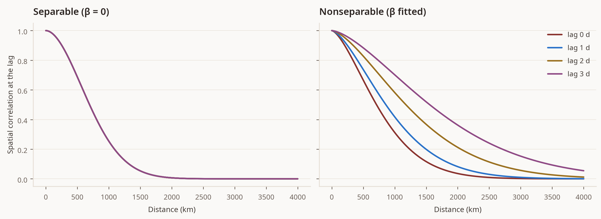
For the separable kernel, the curves are on top of each other: the shape of the spatial correlation does not change with the lag. For the nonseparable kernel, the spatial correlation becomes broader as the lag grows, because only the large anomalies persist from one day to the next.
Notes#
Bounds. The trainable \(\alpha\), \(\beta\) and \(\gamma\) are in the open interval \((0, 1)\). To fix one of them at a bound, pass
paramax.non_trainable(jnp.array(value)), as we did for \(\beta = 0\).Symmetry. The Gneiting kernel is symmetric in space and in time. It cannot represent advection, where anomalies move in one main direction. For daily wind speeds in Ireland (Haslett & Raftery, 1989), which westerly winds carry from west to east, we found no benefit over the separable kernel. Gneiting, Genton & Guttorp (2007) discuss asymmetric models.
Monthly data. Monthly anomalies over Europe showed no interaction: the temporal correlation is shorter than one month, so the time lags carry little information about it.
Pathwise sampling. The kernel has no closed-form spectral density, so
sample_approxdoes not support it. Sample from the predictive distribution instead.
References#
Gneiting, T. (2002). Nonseparable, stationary covariance functions for space–time data. Journal of the American Statistical Association 97, 590–600.
Gneiting, T., Genton, M. G. and Guttorp, P. (2007). Geostatistical space–time models, stationarity, separability and full symmetry. In Statistical Methods for Spatio-Temporal Systems, 151–175. Chapman & Hall/CRC.
Haslett, J. and Raftery, A. E. (1989). Space–time modelling with long-memory dependence: assessing Ireland’s wind power resource. Applied Statistics 38, 1–50.
Kalnay, E. et al. (1996). The NCEP/NCAR 40-year reanalysis project. Bulletin of the American Meteorological Society 77, 437–471.